USER GUIDE

Introduction

T1T2ne is an helper software package to setup protein dynamics ¹⁵N T₁ and T₂and hetNOE experiments. The idea is to save spectrometer time and to optimize the quality of the data, by automatizing the selection of the parametes. The software is executed from command line, and the main entry point is the t1t2ne command. To get a list of available subcommands, you can run:

t1t2ne --help

To get more information on a specific subcommand, you can run:

t1t2ne <subcommand> --help

The following subcommands are available:

• Setup of relaxation experiments

  • interactive: an interactive command line tools that guides the user through the selection of the appropriate parameters for ¹⁵N relaxation measurements.

    See section The interactive subcommand.
  • makelists: a command line tool to generate the lists for running ¹⁵N T₁ and T₂ relaxation experiments given the correlation times or the molecular weight.

    See section The makelists subcommand.
  • ns: a command line tool to estimate the number of scans required for a given experiment, starting from an HSQC experiment.

    See section The ns subcommand.

• Setup and analysis of the TRACT experiment

  • setuptract: a command line tool to set up a TRACT experiment on the spectrometer, providing the appropriate delay list based on the correlation time or molecular weight.

    See section The setuptract subcommand.
  • tract: a command line tool to fit a TRACT experiment and extract the average correlation time of the system.

    See section The tract subcommand.

• Solvent PRE

  • solventpre: a command line tool to generate the lists for running ¹H T₁ and T₂ solvent PRE experiments.

    See section The solventpre subcommand.

Minimal Theoretical Background

We here provide the minimal theoretical background to understand the rationale behind the software. For a more detailed introduction we will provide in-line links to appropriate references. Nuclear spin relaxation processes are caused by the fluctuation of the interactions of the nuclear spin with its environment. Such fluctuations can occur on a range of timescales, hence contribute to different frequencies. This is described through the spectral density functions \(J(\omega)\), which are the Fourier transform of the correlation function of the fluctuating interactions. For proteins, it is common to assume that the spectral density function can be described through the Lipari-Szabo model-free approach, which assumes that the motion of the N-H bond vector can be described through a global reorientation (slow motion) and an internal motion (fast motion). The global reorientation is described through a correlation time \(\tau_c\) and an order parameter \(S^2\), which describes the amplitude of the motion. The internal motion is described through an order parameter \(S^2_f = 1 - S^2\) and a correlation time \(\tau_f\). The resulting spectral density function is then:

\[J(\omega) = \frac{2}{5} \left[ S^2 \frac{\tau_c}{1 + (\omega \tau_c)^2} + (1 - S^2) \frac{\tau_f}{1 + (\omega \tau_f)^2} \right]\]

which, assuming that \(\tau_f\) is of the order of picoseconds, and thus \(\tau_f \ll \tau_c\), can be approximated to:

\[J(\omega) \approx \frac{2}{5} S^2 \frac{\tau_c}{1 + (\omega \tau_c)^2}\]

For Intrinsically Disordered Proteins, several different motional models have been proposed (see Salvi for a review). In this software we have opted for the model proposed by Parigi et al., which assumes that the motion can be described through a slow motion, an intermediate motion and a fast motion. The slow motion is assumed to correspond to the tumbling of a protein of the same size of the one under study, and the order parameter of the slow motion is assumed to be small (e.g., 0.15). The intermediate motion is assumed to have a correlation time of a peptide of 20 residues (1.6 ns). The resulting spectral density function is then:

\[J(\omega) = \frac{2}{5} \left[ S^2_{slow} \frac{\tau_{slow}}{1 + (\omega \tau_{slow})^2} + (1 - S^2_{slow}) S^2_{int} \frac{\tau_{int}}{1 + (\omega \tau_{int})^2} + (1 - S^2_{slow}) (1 - S^2_{int}) \frac{\tau_{fast}}{1 + (\omega \tau_{fast})^2} \right]\]

For a ¹⁵N-¹H pair, the relevant interactions are the dipolar coupling and the chemical shielding anisotropy. The dipolar coupling is described through the constants \(p\) and \(\delta\).

\[p = \frac{\mu_0 h \gamma_H \gamma_N}{16 \pi^2 r^3}\]

\[\delta = -\frac{\Delta \sigma \gamma_N}{3}\]

Where:

• \(\mu_0\) is the vacuum permeability in T m/A

• \(h\) is the Planck constant in J s

• \(\gamma_H\) is the gyromagnetic ratio of the proton in rad/s/T

• \(\gamma_N\) is the gyromagnetic ratio of the nitrogen in rad/s/T

• \(r\) is the distance between the nuclei in meters

• \(\Delta \sigma\) is the anisotropy of the chemical shielding tensor, which is a dimensionless quantity. For a N-H pair, it is around 160 ppm.

The relaxation rates \(R_1\), \(R_2\) and NOE enhancement factor \(\eta\) at a given the magnetic field strength \(B\) can be calculated as reported by Fushman:

\[R_1 = p^2 (J(\omega_H - \omega_N) + 6 J(\omega_H + \omega_N)) + 3 (\delta^2 B^2 + p^2) J(\omega_N)\]

\[R_2 = R_{ex} + \frac{1}{2} p^2 (J(\omega_H - \omega_N) + 6 J(\omega_H + \omega_N) + 6 J(\omega_H)) + \frac{1}{2} (\delta^2 B^2 + p^2) (4 J(0) + 3 J(\omega_N))\]

\[\eta = 1 - \frac{p^2 \gamma_H}{\gamma_N} \frac{6 J(\omega_H + \omega_N) - J(\omega_H - \omega_N)}{R_1}\]

Note

Throughout the code, it is assumed that \(R_{ex}\) is negligible and that also the contribution from neighboring protons is currently neglected.

Given the computed values of \(R_1\), \(R_2\) and \(\eta\), it is possible to compute the an optimal sampling scheme for the experiments, as described by Ferrage.

The use of the symbol \(\eta\) is quite unfortunate, as it also indicates the cross-correlated relaxation rates. For the cross-correlation between the dipolar coupling and the CSA, the rates are reported by Salvi:

\[\eta_z = \frac{1}{15} P_2(\cos\theta) p \delta B 6 J(\omega_X)\]

\[\eta_{xy} = \frac{1}{15} P_2(\cos\theta) p \delta B (4 J(0) + 3 J(\omega_X))\]

where \(\theta\) is the angle between the dipolar coupling and the CSA tensors, which for a N-H pair is around 17 degrees.

Goldman noted that:

\[\eta_{red} = \dfrac{\eta_{xy}}{(3 cos^2 \theta - 1) p d} = 4 J(0) + 3 J(\omega_N)\]

From this relation and from the form of the spectral density function, it is possible to extract the correlation time of the system from the value of \(\eta_{xy}\). This is the rationale behind the TRACT experiment (Lee et al. (2006)). Recently, Robson et al. (2021) have provided a closed-form expression to extract the correlation time from the value of \(\eta_{xy}\) including the possibility to specify a value for the order parameter. The equation is reported in the original paper and is too long to be reproduced here. We note that, while usually not advised, the same reasoning can be applied to extract the order parameter of an IDP:

\[S^2_{int} = \frac{\eta_{red} - 4(S^2_{slow} J(0, \tau_{slow}) + (1-S^2_{slow}) J(0, \tau_{fast})) - 3(S^2_{slow} J(\omega_N, \tau_{slow}) + (1-S^2_{slow}) J(\omega_N, \tau_{fast}))}{4(1-S^2_{slow})(J(0, \tau_{int}) - J(0, \tau_{fast})) + 3(1-S^2_{slow})(J(\omega_N, \tau_{int}) - J(\omega_N, \tau_{fast}))}\]

This closes the circle and allows to have a more robust estimate of the relaxation times and hence to obtain more meaningful delay lists, which in turn gives better experimental data.

Solvent PRE and the Freed Outer Sphere Model

Solvent PRE experiments are based on the fact that the relaxation of a nucleus can be enhanced by the presence of a paramagnetic agent in solution. The effect is distance-dependent, and can be used to obtain information on the solvent accessibility of different residues in a protein. he expected relaxation rates are computed with the Freed Outer Sphere model. In this model, the spectral density function is computed as:

\[\begin{split}\tau_D &= \frac{d^2}{D_{target} + D_{cosolute}} \\ z &= \sqrt{2 |\omega| \tau_D + \frac{\tau_D}{\tau_1}} \\ J_{outer}(\omega) &= \frac{2}{5} \frac{1 + 5 z / 8 + z^2 / 8}{1 + z + z^2/2 + z^3/6 + 4 z^4/81 + z^5/81 + z^6/648}\end{split}\]

where:

• \(d\) is the distance of closest approach of the paramagnetic center and the nucleus in meters

• \(D_{target}\) is the diffusion coefficient of the target molecule in m^2/s

• \(D_{cosolute}\) is the diffusion coefficient of the cosolute molecule in m^2/s

• \(\tau_1\) is the correlation time for electron relaxation in seconds

• \(\omega\) is the angular frequency where the spectral density is evaluated, in rad/s

Equations 6.42, 6.48 and 6.50 in Bertini et al. 2016.

This spectral density function is then used to compute the expected PRE rates, with optional transient zero-field splitting (ZFS) contribution to the electron relaxation. Default values are for 1 mM Gd-DOTA and a protein of 10 kDa at room temperature. The default values correspond to Gd-DOTA, and are taken from Li et al. 2002.

\[\begin{split}k_{outer} = \frac{16\pi}{81} \left( \frac{\mu_0}{4\pi} \right)^2 h^2 \gamma_n^2 \gamma_e^2 S(S+1) f N_A \frac{c}{d(D_{target}+D_{cosolute})}\\ R_1 = k_{outer} [7 J_{outer} (\omega_S) + 3 J_{outer} (\omega_I)]\\ R_2 = \frac{1}{2} k_{outer} [13 J_{outer} (\omega_S) + 3 J_{outer} (\omega_I) + 4 J_{outer} (0)]\end{split}\]

Where:

• \(\mu_0\) is the vacuum permeability in T m/A

• \(h\) is the Planck constant in J s

• \(\gamma_n\) is the gyromagnetic ratio of the nucleus in rad/s/T

• \(\gamma_e\) is the gyromagnetic ratio of the electron in rad/s/T

• \(S\) is the electron spin quantum number

• \(N_A\) is the Avogadro’s number in mol^-1

• \(c\) is the concentration of the paramagnetic cosolute in mol/m^3

• \(f\) is the fraction of the sphere around the nucleus that is accessible to the paramagnetic cosolute.

Optionally, the transient zero-field splitting (ZFS) contribution to electron relaxation is included with the Bloembergen-Morgan model:

\[\begin{split}R_{1e} = \frac{2}{15} \Delta_t^2 \left(4S(S+1) - 3\right) \left(J(\omega_e) + 2J(2\omega_e)\right)\\ R_{2e} = \frac{1}{15} \Delta_t^2 \left(4S(S+1) - 3\right) \left(3J(0) + 5J(\omega_e) + J(2\omega_e)\right)\end{split}\]

Where:

• \(\Delta_t\) is the transient zero-field splitting, provided in inverse centimeters and translated automatically to Hz

• \(\omega_e\) is the electron Larmor frequency in rad/s

Setup of relaxation experiments

Getting started on a spectrometer workstation

This section describes the recommended first-time setup of T1T2ne on a Bruker TopSpin spectrometer workstation. The goal is to let the software automatically discover instrument parameters (e.g. field strength) and to store a default dataset location that can be reused by the TRACT and NS modules.

The workflow has two phases:

1. One-time configuration (performed by an NMR superuser).

2. Day-to-day usage (performed by any user running t1t2ne).

Warning

The command t1t2ne configure writes a configuration file inside the TopSpin installation (in the prog/curdir/<user>/ area). For this reason it can only be run by a user listed in the TopSpin nmrsuperuser file. If you are not a superuser, ask the local NMR facility staff to run the configuration step once.

Prerequisites

• Python >= 3.10 must be available on the workstation.

• TopSpin must be installed locally on the workstation.

• For the configuration step only: you must be an NMR superuser (TopSpin admin).

Installation (NMR superuser)

Install the software as described in the `Installation guide`_. On a linux workstation, we have installed miniconda in the /opt/miniconda3 directory, and then installed T1T2ne in a conda environment named t1t2ne with the command:

conda create --name t1t2ne python=3.10
conda activate t1t2ne
pip install t1t2ne

At the end of the installation, for each user, you can initialize conda and the enviroment with:

/opt/miniconda3/bin/conda init bash
conda activate t1t2ne

One-time configuration (NMR superuser)

Run the configuration command from a terminal:

t1t2ne configure

The program will:

• locate the local TopSpin installation (or you can provide it explicitly, see below),

• ask for a standard dataset directory (a dataset you want to use as default example/reference),

  • can be specified with --basedir (dataset directory),

• ask for the experiment number of a TRACT experiment

  • can be specified with - --tract (TRACT experiment number),

• verify that the selected TRACT experiment is actually a TRACT experiment (by inspecting the pulse program name),

• ask for the experiment number of an HSQC experiment within that dataset,

  • can be specified with --hsqc (HSQC experiment number, used by the ns module).

• write a configuration file named tract_analysis_config.ini in the TopSpin curdir for the current user.

Note

curdir is a TopSpin concept that refers to a user-specific directory which is carried over across successive TopSpin installations.

The resulting config is used by T1T2ne to pre-fill the default values for dataset location and experiment numbers for the test datasets, to be used as a reference for the users.

If TopSpin is not found automatically, or if you want to force a specific path, you can provide it:

t1t2ne configure --topspinpath /opt/topspin4

(Replace the path with the local TopSpin installation directory on your system.)

Day-to-day usage on the spectrometer

Once the configuration file exists, most commands can be run with minimal arguments, because the software will reuse the defaults recorded in tract_analysis_config.ini.

Troubleshooting

Problem: TopSpin does not appear to be installed on this workstation Cause: T1T2ne could not locate TopSpin. Fix: run t1t2ne configure --topspinpath <path> (superuser) or contact facility staff.

Problem: Only the NMR superuser can write the config file. Exiting. Cause: you are not listed in TopSpin nmrsuperuser. Fix: ask facility staff (superuser) to run t1t2ne configure once.

Problem: Experiment <N> is not a TRACT experiment Cause: the selected experiment does not appear to be a TRACT dataset (based on pulse program inspection). Fix: double-check the experiment number and confirm the TRACT sequence name used on your system contains the substring tract.

The interactive subcommand

Warning

The interactive subcommand requires to be run on a spectrometer workstation. The other subcommands can be run on any computer, included personal and processing stations.

This subcommand uses the name scheme of the two pulse sequences for T₁ and T₂ measurements provided with this package (hsqct1etf3gptcwg1d.rav and hsqct2etf3gptcwg1d.rav).

Let us assume we have a protein of 8.6 kDa (ubiquitin) and we want to measure T₁ and T₂ at 600 MHz.

• The first experiment to be set up is the T₁. Set the sequence to hsqct1etf3gptcwg1d.rav.

• Calling the interactive subcommand as:

  t1t2ne interactive --MW 8.6 --Larmor 600
  

  will provide the user with the maximum expected delay (d29), and prompt to acquire a reference experiment with a short delay (d31 = 20 us). The longest delay is used for temperature compensation.

• After acquiring the reference experiment, the user is prompted to provide the experiment number of the reference, phase it, and select the integration region. The instructions on how to use the GUIs can be found in klassez.processing.interactive_phase_1D() and klassez.anal.integrate() respectively.

  The software will then provide an estimate for d31 as the one that provides a reduction to about 30% of the reference intensity.

  Note

  This is the value that maximizes the Fisher Information criterium for a single exponential decay.

• After the user has acquired the T₁ experiment with the suggested delay, the software will integrate it in the same region provide a new estimate for the delay. The process is repeated until the obtained value falls within 10% of the suggested value.

With the obtained T₁ value, also the suggested interscan delay for the hetNOE experiment is provided.

The same process is then repeated for the T₂ experiment, using the sequence hsqct2etf3gptcwg1d.rav and setting the l29 and l31 to the suggested initial values. The only difference in this procedure is that the software will NEVER suggest to acquire a T₂ experiment with total CPMG time with a duty cycle larger than 250 ms with the Bruker library settings, to avoid damage to probe, or sample, or spectrometer hardware.

The software accepts several command line options to customize the procedure:

• Parameters related to the acquisition of the experiments:

  • --basedir: the base directory of the experiments. This overrides the default current directory. If not set, the user will be prompted to enter it at the beginning of the procedure. The software will check that the specified directory exists.

  • --xred: the percent residual signal for the longest delay of the experiments. If not set, it will defaulto to 5% and 10% for T₁and T₂ respectively.

  • --nT: the number of increments in the suggested vdlist for the T₁ experiment and T₁ T₂ experiments. Default is 8. If more than one value is provided, the first one will be used for the T₁ experiment, and the second one for the T₂ experiment.

  • --logscale: whether to use a logarithmic scale for the vdlist and vclist. Default is False, which means a linear scale will be used.

  • --randomize: whether to randomize the order of the values in the lists. Default is False.

  • --Larmor: the Larmor frequency of the spectrometer, in MHz. It will anyway be read from the configuration file of the spectrometer.

  • --B0: the magnetic field strength of the spectrometer, in Tesla. It will anyway be read from the configuration file of the spectrometer.

  • --large: whether to create the lists for the “large” sequence, which is optimized for short T2 times. Default is False.

  • --small: whether to create the lists for the “small” sequence, which is optimized for long T2 times. Default is False.

• Parameters related to the estimation of the correlation times and order parameters:

  • --S2: the Lipari-Szabo order parameter S2 to use for the calculation of tau_c. In IDP mode, two values should be provide, else only one

  • --MW: the molecular weight of the protein in kDa, to be used for estimating the longest correlation time (tau_slow in the IDP model).

  • --tau: the correlation times to use for the estimation of the initial delays. In IDP mode, two values should be provided, else only one. If not set, they will be estimated from the MW. Otherwise, default T₁and T₂ values will be used for the non-IDP model, and the three-tau model described in Rezaei-Galeh et al. for the IDP model.

  • --idp: whether the system under study is an intrinsically disordered protein (IDP). If set, the software will use the three-tau model described above. Default is False.

    • If set, it will also select a longer delay in the cpmg for the T₂ experiment, optimized for the expected relaxation behavior of IDPs as described by Bolognesi et al..

    • If set, it will also select a longer delay for the T₁ experiment, to avoid excessive heating, because cross-correlations are less important in IDPs.

    • the --MW argument will be used to compute the slowest correlation time.

    • --corr_window_idp: the length of the correlation window for the IDP model, in residues. Default is 20.

  • --T: the temperature in Kelvin, to be used for estimating the taus from MW. Default is 298 K.

• Parameters related to relaxation:

  • --r: the length of the 1H-15N bond in Angstroms. Default is 1.02 A.

  • --Deltasigma: the chemical shift anisotropy of the 15N nucleus in ppm. Default is -160 ppm.

  • --nucs: the nuclei to use for the calculation of the relaxation rates. Default is 1H and 15N.

See also

t1t2ne.scripts.t1t2ne_interactive

The makelists subcommand

The scope of this subcommand is generally the same as the The interactive subcommand, i.e.: it generates the lists for running ¹⁵N T₁ and T₂ relaxation experiments given the correlation times or the molecular weight. At variance with the The interactive subcommand, however, it does not provide an interactive procedure to optimize the delays. For this reason, it is recommended to be used after the The tract subcommand experiment, to generate the lists for the final acquisition of the experiments with the optimized delays (see below). As for the The interactive subcommand, this subcommand uses the name scheme of the two pulse sequences for T₁ and T₂ measurements provided with this package (hsqct1etf3gptcwg1d.rav and hsqct2etf3gptcwg1d.rav).

It is called as:

t1t2ne makelists --MW 8.6 --Larmor 600

Which will generate the following output:

$ t1t2ne makelists --MW 8.6 --Larmor 600

**************************************************
*                                                *
*                  T-one-T-tune                  *
*                                                *
*                makelists module                *
*                                                *
**************************************************
*                 Main Author:                   *
*                                                *
*                 Enrico Ravera                  *
*                                                *
*      Dipartimento di Chimica "Ugo Schiff"      *
*             University of Florence             *
*                                                *
*                       &                        *
*                                                *
*          Consorzio Interuniversitario          *
*    Risonanze Magnetiche di Metalloproteine     *
*                                                *
*                 Contributors:                  *
*                Francesco Bruno                 *
*                                                *
*                Letizia Fiorucci                *
**************************************************

No value provided for the xred parameter. Defaulting to [10, 30].
TopSpin does not appear to be installed on a spectrometer workstation.
Config file not found in the curdir folder of topspin for any of the users in the nmrsuperuser list.


Estimated values for heteronuclear relaxation:

expected T1 = 0.507 s
expected T2 = 0.132 s
expected hetnOe = 0.784
Set the recovery delay for the hetnOe experiment in the range 2.026 - 3.039.

Creating vdlist with 8 points and vclist with 8 points...


The longest delay for the T1 experiment for a residual signal of 10% should be 1.17 s.

vdlist for T1 experiment:
-------------------------
20.00u
0.17000
0.33000
0.50000
0.67000
0.83000
1.00000
1.17000
Enter the d21 value in microseconds (default 450):
Enter the p30 value in microseconds (default 160):
With the chosen d21 and p30 values, the maximum CPMG block allowed by the duty cycle is 0.25 s.
Warning: the second CPMG point in logscale would be a repetition of the first, switching to "large" sequence
The longest CPMG block for T2 for a residual signal of 30% should be 0.16 s, with 18 loops.
Check if this is too long for your equipment before running the experiment

vclist for T2 experiment:
-------------------------
0
2
5
7
10
12
15
18



*****************************************************

Analysis complete. Below are the references for the methods used in this software.
We can not nor we want to force you to cite any of these papers, but we - and likewise (we believe) the authors of the original papers - appreciate if you do.
- Cavanagh, J., Fairbrother, W. J., Palmer III, A. G., Rance, M., & Skelton, N. J. (2007). Protein NMR spectroscopy: principles and practice. Academic Press. DOI: 10.1016/B978-0-12-164491-8.X5000-3

- Fushman, D. (2012). Determining Protein Dynamics from 15N Relaxation Data by Using DYNAMICS. In: Shekhtman, A., Burz, D. (eds) Protein NMR Techniques. Methods in Molecular Biology, vol 831. Humana Press. DOI: 10.1007/978-1-61779-480-3_24

*****************************************************

If the IDP model is selected, the output will be similar:

t1t2ne makelists --MW 14.4 --Larmor 600 --idp

Which will provide the following output:

$ t1t2ne makelists --MW 14.4 --Larmor 600 --idp

**************************************************
*                                                *
*                  T-one-T-tune                  *
*                                                *
*                makelists module                *
*                                                *
**************************************************
*                 Main Author:                   *
*                                                *
*                 Enrico Ravera                  *
*                                                *
*      Dipartimento di Chimica "Ugo Schiff"      *
*             University of Florence             *
*                                                *
*                       &                        *
*                                                *
*          Consorzio Interuniversitario          *
*    Risonanze Magnetiche di Metalloproteine     *
*                                                *
*                 Contributors:                  *
*                Francesco Bruno                 *
*                                                *
*                Letizia Fiorucci                *
**************************************************

No value provided for the xred parameter. Defaulting to [10, 30].
TopSpin does not appear to be installed on a spectrometer workstation.
Config file not found in the curdir folder of topspin for any of the users in the nmrsuperuser list.


Estimated values for heteronuclear relaxation:

expected T1 = 1.091 s
expected T2 = 0.349 s
expected hetnOe = 0.390
Set the recovery delay for the hetnOe experiment in the range 4.363 - 6.544.

Creating vdlist with 8 points and vclist with 8 points...


The longest delay for the T1 experiment for a residual signal of 10% should be 2.51 s.

vdlist for T1 experiment:
-------------------------
20.00u
0.36000
0.72000
1.08000
1.44000
1.80000
2.16000
2.52000
Using ".idp" sequence, which is optimized for long T2 times. d21 = 750u
Enter the d21 value in microseconds (default 750):
Enter the p30 value in microseconds (default 160):
With the chosen d21 and p30 values, the maximum CPMG block allowed by the duty cycle is 0.64 s.
Warning: the CPMG block of 0.03 s is too long for the T2 timescale, switching off the  "small" option
The longest CPMG block for T2 for a residual signal of 30% should be 0.42 s, with 24 loops.
Check if this is too long for your equipment before running the experiment

vclist for T2 experiment:
-------------------------
0
3
6
10
13
17
20
24



*****************************************************

Analysis complete. Below are the references for the methods used in this software.
We can not nor we want to force you to cite any of these papers, but we - and likewise (we believe) the authors of the original papers - appreciate if you do.
- Cavanagh, J., Fairbrother, W. J., Palmer III, A. G., Rance, M., & Skelton, N. J. (2007). Protein NMR spectroscopy: principles and practice. Academic Press. DOI: 10.1016/B978-0-12-164491-8.X5000-3

- Rezaei‐Ghaleh, N., Parigi, G., Soranno, A., Holla, A., Becker, S., Schuler, B., ... & Zweckstetter, M. (2018). Local and global dynamics in intrinsically disordered synuclein. Angewandte Chemie International Edition, 57(46), 15262-15266. DOI: 10.1002/anie.201808172

- Fushman, D. (2012). Determining Protein Dynamics from 15N Relaxation Data by Using DYNAMICS. In: Shekhtman, A., Burz, D. (eds) Protein NMR Techniques. Methods in Molecular Biology, vol 831. Humana Press. DOI: 10.1007/978-1-61779-480-3_24

*****************************************************

As mentioned earlier, this script is more appropriately run following the a TRACT experiment. Taking as example the ubiquitin data described below in The tract subcommand:

t1t2ne makelists --tau 4.57e+00 --S2 0.90 --Larmor 600

Likewise, after the synuclein TRACT experiment described in The tract subcommand:

t1t2ne makelists --tau 8.80e+00 1.49e+00 --S2 0.15 0.38 --Larmor 600

The software accepts several command line options to customize the procedure:

• Parameters related to the acquisition of the experiments:

  • --xred: the percent residual signal for the longest delay of the experiments. If not set, it will defaulto to 5% and 10% for T₁and T₂ respectively.

  • --nT: the number of increments in the suggested vdlist for the T₁ experiment and T₁ T₂ experiments. Default is 8. If more than one value is provided, the first one will be used for the T₁ experiment, and the second one for the T₂ experiment.

  • --logscale: whether to use a logarithmic scale for the vdlist and vclist. Default is False, which means a linear scale will be used.

  • --randomize: whether to randomize the order of the values in the lists. Default is False.

  • --Larmor: the Larmor frequency of the spectrometer, in MHz. It will anyway be read from the configuration file of the spectrometer.

  • --B0: the magnetic field strength of the spectrometer, in Tesla. It will anyway be read from the configuration file of the spectrometer.

  • --large: whether to create the lists for the “large” sequence, which is optimized for short T2 times. Default is False.

  • --small: whether to create the lists for the “small” sequence, which is optimized for long T2 times. Default is False.

• Parameters related to the estimation of the correlation times and order parameters:

  • --S2: the Lipari-Szabo order parameter S2 to use for the calculation of tau_c. In IDP mode, two values should be provide, else only one

  • --MW: the molecular weight of the protein in kDa, to be used for estimating the longest correlation time (tau_slow in the IDP model).

  • --tau: the correlation times to use for the estimation of the initial delays. In IDP mode, two values should be provided, else only one. If not set, they will be estimated from the MW. Otherwise, default T₁and T₂ values will be used for the non-IDP model, and the three-tau model described in Rezaei-Galeh et al. for the IDP model.

  • --idp: whether the system under study is an intrinsically disordered protein (IDP). If set, the software will use the three-tau model described above. Default is False.

    • If set, it will also select a longer delay in the cpmg for the T₂ experiment, optimized for the expected relaxation behavior of IDPs as described by Bolognesi et al..

    • If set, it will also select a longer delay for the T₁ experiment, to avoid excessive heating, because cross-correlations are less important in IDPs.

    • the --MW argument will be used to compute the slowest correlation time.

    • --corr_window_idp: the length of the correlation window for the IDP model, in residues. Default is 20.

  • --T: the temperature in Kelvin, to be used for estimating the taus from MW. Default is 298 K.

• Parameters related to relaxation:

  • --r: the length of the 1H-15N bond in Angstroms. Default is 1.02 A.

  • --Deltasigma: the chemical shift anisotropy of the 15N nucleus in ppm. Default is -160 ppm.

  • --nucs: the nuclei to use for the calculation of the relaxation rates. Default is 1H and 15N.

See also

t1t2ne.scripts.t1t2ne_makelists

The ns subcommand

This subcommand estimates the number of scans required for a given experiment, starting from an HSQC experiment. There are two ways the estimate of SNR is done:

1. By direct estimation of the SNR from the 2D spectrum using klassez.anal.snr().

2. By estimating the SNR from the envelope of the first transient of the TRACT experiment, and using the expected linewidh and the number of resonances to compute the expected intensity for a single peak.

In both cases the user needs to provide the path to an experiment to analyze through the parameters basedir and either hsqc or tract. If for instance the dataset is in /path/to/my/dataset/42, these arguments should be passed as --basedir /path/to/my/dataset --hsqc 42. The expected reduction in intensity for the experiment to be setup with respect to this reference HSQC should be passed as a percentage value through the argument xred. The calculation is performed for each entry of the --xred argument list. The first method is more accurate, but requires the user to have already acquired an HSQC spectrum of the sample, using the same parameters (type of sequence, number of transients) as those for relaxation. This is used with:

t1t2ne ns --basedir <basedir> --hsqc <HSQC experiment number> --xred 10 30 70 --snr2d

The number of scans is estimated for each entry of the xred list, assuming that only <xred>% of the intensity of the peaks in the reference HSQC will be observed in the relaxation experiments. The SNR per scan is estimated from the SNR value of the 2D spectrum and the status <ns> of the same experiment, and then the number of scans required to reach a SNR of 10 at the <xred>% intensity is estimated. Finally, the results are printed out rounding to the nearest multiple of 4 for the hetNOE experiment, and to the nearest multiple of 8 for the T₁ and T₂ experiments to respect phase cycling. The second method is intrinsically less accurate, but the guess is still within a decent ballpark, and it can be used even before acquiring any 2D spectrum of the sample. Taking as example a protein of 8.6 kDa (ubiquitin), the script is invoked by typing:

t1t2ne ns --MW 8.6 --basedir <basedir> --tract <TRACT experiment number> --xred 10 30 70

The algorithm works as follows:

1. The provided spectrum is phased and the first transient is integrated.

2. The number of signals under the integrated region are either counted on the basis of the MW, or provided by the user.

3. The SNR for each signal is then estimated.

4. The number of scans required to reach a SNR of 10 (the conventional quantitativity limit) at the longest delay (i.e. the worst case) is estimated.

5. The number of scans is rounded to the nearest multiple of 4 for the hetNOE experiment, and to the nearest multiple of 8 for the T₁ and T₂ experiments to respect phase cycling.

See also

t1t2ne.scripts.t1t2ne_ns klassez.anal.snr()

Setup and analysis of the TRACT experiment

The setuptract subcommand

This subcommand generates the delay list for running a TRACT experiment on the spectrometer, providing the appropriate delay list based on the correlation time or molecular weight. The general syntax for this command is the following:

t1t2ne setuptract --MW <MW> --Larmor <Frequency in MHz>

The rationale is the same as for the makelists subcommand (see The makelists subcommand), where the correlation times of the system are either provided by the user or computed from the molecular weight, and the relaxation rates computed accordingly. The the Larmor frequency of ¹H at the given field is needed unless the program is run on the spectrometer, in which case this information is not needed, as it is direcly taken from there.

The software will then generate a delay list for the TRACT experiment that covers a range of delays that is appropriate for the expected correlation time, and that maximizes the Fisher Information criterium for matching the decay rates of both \(\alpha\) and \(\beta\) components of the TROSY.

See also

t1t2ne.scripts.t1t2ne_setuptract

Examples

If I have a 8.6 kDa protein (ubiquitin) and a 600 MHz spectrometer, the script should be invoked as:

• Case 1: I know the Molecular Weight and I am at the spectrometer computer

  t1t2ne setuptract --MW 8.6
  

• Case 2: I know the correlation time and I am at the spectrometer computer

  t1t2ne setuptract --tauc 66.6
  

• Case 3: I know the Molecular Weight and I am not at the spectrometer computer

  t1t2ne setuptract --MW 8.6 --Larmor 600
  

• Case 4: I know the correlation time and I am not at the spectrometer computer

  t1t2ne setuptract --tauc 66.6 --Larmor 600
  

In any case, the software will generate a delay list for the TRACT experiment that covers a range of delays that is appropriate for the expected correlation time, and that maximizes the Fisher Information criterium for matching the decay rates of both \(\alpha\) and \(\beta\) components of the ¹H- ¹⁵N doublet.

The output looks like this:

$ t1t2ne setuptract --MW 6.2 --Larmor 600

**************************************************
*                                                *
*                  T-one-T-tune                  *
*                                                *
*               setuptract module                *
*                                                *
**************************************************
*                 Main Author:                   *
*                                                *
*                 Enrico Ravera                  *
*                                                *
*      Dipartimento di Chimica "Ugo Schiff"      *
*             University of Florence             *
*                                                *
*                       &                        *
*                                                *
*          Consorzio Interuniversitario          *
*    Risonanze Magnetiche di Metalloproteine     *
*                                                *
*                 Contributors:                  *
*                Francesco Bruno                 *
*                                                *
*                Letizia Fiorucci                *
**************************************************

TopSpin does not appear to be installed on this workstation.
Config file not found in the curdir folder of topspin for any of the users in the nmrsuperuser list.

Calculating the optimal vdlist for the TRACT experiment...

Provided parameters:
Correlation time(s): [3.8861600000000006e-09, 1e-11] s
Order parameter(s) S2: [0.9]

Estimated relaxation rates:
R1:  2.32 s^-1, R2: 5.98 s^-1, nOe: 0.75
Ra:  1.56 s^-1
Rb:  10.40 s^-1

Suggested vdlist for TRACT experiment:
--------------------------------------
10.00u
50.34u
253.40u
1.28m
6.42m
0.06144
0.40955
0.81909

*****************************************************

Analysis complete. Below are the references for the methods used in this software.
We can not nor we want to force you to cite any of these papers, but we - and likewise (we believe) the authors of the original papers - appreciate if you do.
- Cavanagh, J., Fairbrother, W. J., Palmer III, A. G., Rance, M., & Skelton, N. J. (2007). Protein NMR spectroscopy: principles and practice. Academic Press. DOI: 10.1016/B978-0-12-164491-8.X5000-3

- Lee, D., Hilty, C., Wider, G., Wüthrich, K. (2006). J. Magn. Reson., 178, 72-76 DOI: 10.1016/j.jmr.2005.08.014

- Fushman, D. (2012). Determining Protein Dynamics from 15N Relaxation Data by Using DYNAMICS. In: Shekhtman, A., Burz, D. (eds) Protein NMR Techniques. Methods in Molecular Biology, vol 831. Humana Press. DOI: 10.1007/978-1-61779-480-3_24

- Salvi, N., Abyzov, A., Blackledge, M. (2017). Atomic resolution conformational dynamics of intrinsically disordered proteins from NMR spin relaxation. Progress in Nuclear Magnetic Resonance Spectroscopy, 102-103, 43-60. DOI: 10.1016/j.pnmrs.2017.06.001

*****************************************************

The software accepts several command line options to customize the procedure:

• Parameters related to the acquisition of the experiments:

  • --nT: the number of increments in the suggested vdlist. Default is 8. If more than one value is provided, the first one will be used and the others will be discarded.

  • --randomize: whether to randomize the order of the values in the lists. Default is False.

  • --Larmor: the Larmor frequency of the spectrometer, in MHz. It will be read from the configuration file of the spectrometer.

  • --B0: the magnetic field strength of the spectrometer, in Tesla. It will be read from the configuration file of the spectrometer.

• Parameters related to the estimation of the correlation times and order parameters:

  • --S2: the Lipari-Szabo order parameter S2 to use for the calculation of tau_c. In IDP mode, two values should be provide, else only one

  • --MW: the molecular weight of the protein in kDa, to be used for estimating the longest correlation time (tau_slow in the IDP model).

  • --tau: the correlation times to use for the estimation of the initial delays. In IDP mode, two values should be provided, else only one. If not set, they will be estimated from the MW. Otherwise, default T₁and T₂ values will be used for the non-IDP model, and the three-tau model described in Bolognesi et al. for the IDP model.

  • --idp: whether the system under study is an intrinsically disordered protein (IDP). If set, the software will use the three-tau model described above. Default is False.

    • If set, it will also select a longer delay in the cpmg for the T₂ experiment, optimized for the expected relaxation behavior of IDPs as described by Bolognesi et al..

    • If set, it will also select a longer delay for the T₁ experiment, to avoid excessive heating, because cross-correlations are less important in IDPs.

    • the --MW argument will be used to compute the slowest correlation time.

    • --corr_window_idp: the length of the correlation window for the IDP model, in residues. Default is 20.

  • --T: the temperature in Kelvin, to be used for estimating the taus from MW. Default is 298 K.

• Parameters related to relaxation:

  • --r: the length of the 1H-15N bond in Angstroms. Default is 1.02 A.

  • --Deltasigma: the chemical shift anisotropy of the 15N nucleus in ppm. Default is -160 ppm.

  • --theta: the angle between the 1H-15N bond and the principal axis of the CSA tensor in degrees. Default is 17 degrees.

  • --nucs: the nuclei to use for the calculation of the relaxation rates. Default is 1H and 15N.

The tract subcommand

This subcommand fits a TRACT experiment and extracts the correlation time of the system either averaged if the flag –integrate is used, or across the spectrum. It uses the algebraic analysis described in Robson et al. (2021), and that is available on GitHub as nomadiq/TRACT_analysis.

The script is invoked as:

t1t2ne tract --basedir <basedir> --tract <TRACT experiment number> --integrate

The TRACT experiment to analyzed is interpreted to be in the <basedir>/<TRACT experiment number> directory.

Note

The user must provide the experiment number of the TRACT experiment. If not provided, the software will look for the configuration file. If it is not found, it will fall back on the examples directory.

The algorithm works as follows.

• The software will load the spectrum and process it.

• phase it using the interactive phasing GUI (see klassez.processing.interactive_phase_1D()).

  • If the flag –integrate is used, the user will be prompted to select the region of the spectrum to be integrated using the interactive integration GUI (see klassez.anal.integrate()).

  • Else, the software will select the region of the spectrum to be fitted.

    • using the flag –selectregion the user will be prompted to select it using the interactive integration GUI (see klassez.fit.get_region()).

    • else, the software will select the NH region of the spectrum to be fitted ([8.6, 7.4] ppm for idps and [10, 7] ppm for globular proteins).

• The decay curves obtained from the integrated regions are then fitted to extract the relaxation rates of the TROSY and the AntiTROSY components.

• The rates are subtracted to extract the cross-correlation rate, and the correlation time is extracted from it using the algebraic analysis described in Robson et al. (2021).

• The values can be visualized as function of the position in the spectrum by providing the --plot argument.

For ubiquitin at 600 MHz, the call is, for instance

t1t2ne tract --basedir <basedir> --tract <TRACT experiment number> --selectregion --plot

—

The results are shown in the following figure.

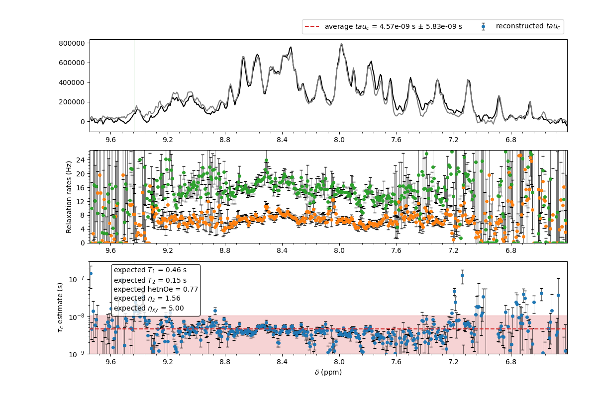
The result of the TRACT analysis for ubiquitin at 600 MHz in the --selectregion mode. The raw data are provided in the examples directory.

At variance with the original paper (Robson et al. (2021)), we foresee the use for Intrinsically Disordered Proteins (IDPs). When the --idp option is used, the software will NOT compute the correlation time but the order parameter \(S^2_{int}\) of the intermediate motion.

In this case the call is, for instance for synuclein at 600 MHz:

t1t2ne tract --basedir <basedir> --tract <TRACT experiment number> --idp --MW 14.4 --selectregion --plot

The results are shown in the following figure.

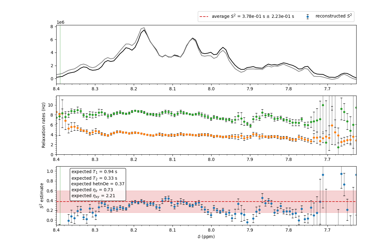
The result of the TRACT analysis for the IDP synuclein at 600 MHz in the --selectregion mode. The raw data are provided in the examples directory.

At the end of the analysis, the software provides the command to generate the lists for running T₁ and T₂ experiments based on the obtained correlation time.

Solvent PRE

The solventpre subcommand

This subcommand generates the lists for running \(^1\) H T₁ and T₂ solvent PRE experiments. T It can be called providing only the field as:

t1t2ne solventpre --Larmor 600

Alternatively, the user can provide the expected intrinsic T₁ of the system and/or the expected linewidth:

t1t2ne solventpre --Larmor 600 --T1 1 --lw 10

The expected linewidth can also be estimated from the molecular weight of the system:

t1t2ne solventpre --Larmor 600 --MW 8.6

By default, the software will suggest a list of 8 delays for T₁ and 2 points for T₂, as described by Iwahara, Tang, and Clore in 10.1016/j.jmr.2006.10.003. The number of points can be changed with the --nT argument.

Important: The delays are calculated under the assumption that the pulse sequence used for T₂ is the one found in figure 1 of 10.1016/j.jmr.2006.10.003.:

Acknowledgements

This software has been developed in the context of the project “TiReD: Time-resolved magnetic resonance to investigate dynamic events in biological systems and biotransformations”, funded by the Ministero dell’Università e della Ricerca (MUR) in the framework of the PRIN 2022 program / Next Generation EU (Bando Prin 2022 - Decreto Direttoriale n. 104 del 02-02-2022 2022WANFH5 CUP: B53D23013990006).

Besides the development team (Enrico Ravera, Francesco Bruno, and Letizia Fiorucci), this software has been developed with the contribution of:

• Marco Schiavina - UniFI - Testing and conceptualization

• Massimo Lucci - CIRMMP - Technical support, testing and conceptualization

We would like to thank the CERM/CIRMMP staff who suggested features and tested the software, in particular:

• Linda Cerofolini - UniFI - Testing and suggestions

• Giacomo Parigi - UniFI - Discussion on relaxation theory

We also thank the master student Petra Vukovic from the University of Zagreb, visiting our lab under the Erasmus+ traineship program for testing the software.

In addition, we would like to mention that the idea for developing this software came from a staff exchange visit between CIRMMP and LIOS as a part of the MRLatvia project.